- Generative and discriminative models
- Naive Bayes classifier
- Feature Representations
- Logistic Regression
- Representing Text with a RNN
- Convolutional Neural Network
Generative and discriminative models
Generative (joint) models \(P(c, d)\)
- Model the distribution of individual classes and place probabilities over both observed data and hidden variables (such as labels)
- E.g. n-gram models, hidden Markov models, probabilistic context-free grammars, IBM machine translation models, Naive Bayes...
Discriminative (conditional) models \(P(c|d)\)
- Learn boundaries between classes. Take data as given and put probability over the hidden structure give the data.
- E.g. logistic regression, maximum entropy models, conditional random fields, support-vector machines...
Naive Bayes classifier
Bayes' Rule: \[ P(c|d) = \frac{P(c)P(d|c)}{P(d)} \] This estimates the probility of document \(d\) being in class \(c\), assuming document length \(n_d\) and tokens \(t\): \[ P(c|d) = P(c)P(d|c) = P(c)\prod_{1 ≤i≤n_d}P(t_i|c) \] Independence Assumptions
Note that we assume \(P(t_i|c) = P(t_j|c)\) independent of token position. This is the naive part of Naive Bayes.
The best class is the maximum a posteriori (MAP) clss: \[ c_{map} = \arg\max_{c\in C}P(c|d) = \arg\max_{c\in C}P(c)\prod_{1≤i≤n_d}P(t_i|c) \] Multiplying tons of small probabilities is tricky, so log space it: \[ c_{map} = \arg\max_{c\in C}(\log P(c) + \sum_{1≤i≤n_d}\log P(t_i|c)) \] Finally: zero probabilities are bad. Add smoothing: \[ P(t|c) = \frac{T_{ct}}{\sum_{t'\in V}T_{ct'}} => P(t|c) = \frac{T_{ct} + 1}{\sum_{t'\in V}T_{ct'}+|V|} \] This is Laplace or add-1 smoothing.
Advantages
- Simple
- Interpretable
- Fast (linear in size of training set and test document)
- Text representation trivial (bag of words)
Drawbacks
- Independence assumptions often too strong
- Sentence/document structure not taken into account
- Naive classifier has zero probabilities; smoothing is awkward
Naive Bayes is a generative model!!! \[ P(c|d)P(d) = P(d|c)P(c) = P(d, c) \] While we are using a conditional probability \(P(c|d)\) for classification, we model the joint probability of \(c\) and \(d\).
This meas it is trivial to invert the process and generate new text given a class label.
Feature Representations
A feature representation (of text) can be viewed as a vector where each element indicates the presence or absence of a given feature in a document.
Note: features can be binary (presence/absence), multinomial (count) or continuous (eg. TF-IDF weighted).
Logistic Regression
A general framework for learning \(P(c|d)\) is logistic regression
- logistic : because is uses a logistic function
- regression : combines a feature vector (\(d\)) with weights (\(\beta\)) to compute an answer
Binary case: \[ P(true|d) = \frac{1}{1 + \exp(\beta_0 + \sum_i\beta_iX_i)} \]
\[ P(false|d) = \frac{\exp(\beta_0 + \sum_i\beta_iX_i)}{1 + \exp(\beta_0+\sum_i\beta_iX_i)} \]
Multinomial case: \[ P(c|d) = \frac{\exp(\beta_{c,0} + \sum_i\beta_{c,i}X_i)}{\sum_{c'}\exp(\beta_{c',0} + \sum_i\beta_{c',i}X_i)} \] The binary and general functions for the logistic regression can be simplified as follows: \[ P(c|d) = \frac{1}{1+\exp(-z)} \]
\[ P(c|d) = \frac{\exp(z_c)}{\sum_{c'}\exp(z_{c'})} \]
which are referred to as the logistic and softmax function.
Given this model formulation, we want to learn parameters \(β\) that maximise the conditional likelihood of the data according to the model.
Due to the softmax function we not only construct a classifier, but learn probability distributions over classifications.
There are many ways to chose weights \(β\):
- Perceptron Find misclassified examples and move weights in the direction of their correct class
- Margin-Based Methods such as Support Vector Machines can be used for learning weights
- Logistic Regression Directly maximise the conditional log-likelihood via gradient descent.
Advantages
- Still reasonably simple
- Results are very interpretable
- Do not assume statistical independence between features!
Drawbacks
- Harder to learn than Naive Bayes
- Manually designing features can be expensive
- Will not necessarily generalise well due to hand-craftedfeatures
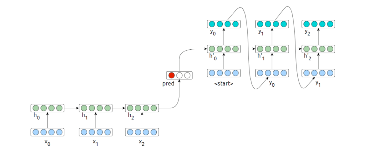
Representing Text with a RNN
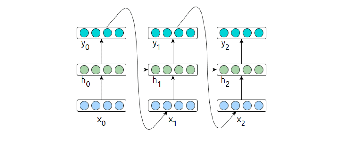
- \(h_i\) is a function of \(x\{0:i\}\) and \(h\{0:i−1\}\)
- It contains information about all text read up to point \(i\).
- The first half of this lecture was focused on learning a representation \(X\) for a given text
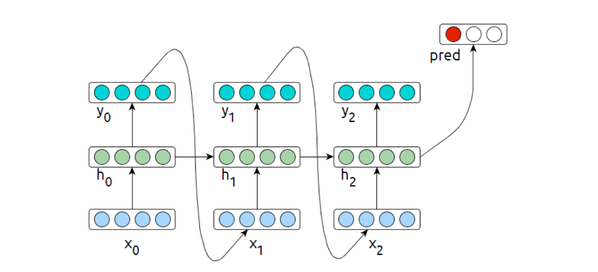
So in order to classify text we can simply take a trained language model and extract text representations from the final hidden state \(c_n\).
Classification as before using a logistic regression: \[ P(c|d) = \frac{\exp(\beta_{c,0} + \sum_i\beta_{c,i}h_{ni})}{\sum_{c'}\exp(\beta_{c',0} + \sum_i\beta_{c',i}h_{ni})} \] ✅ Can use RNN + Logistic Regression out of the box ✅ Can in fact use any other classifier on top of \(h\) ! ❌ How to ensure that \(h\) pays attention to relevant aspects of data?
Move the classification function inside the network
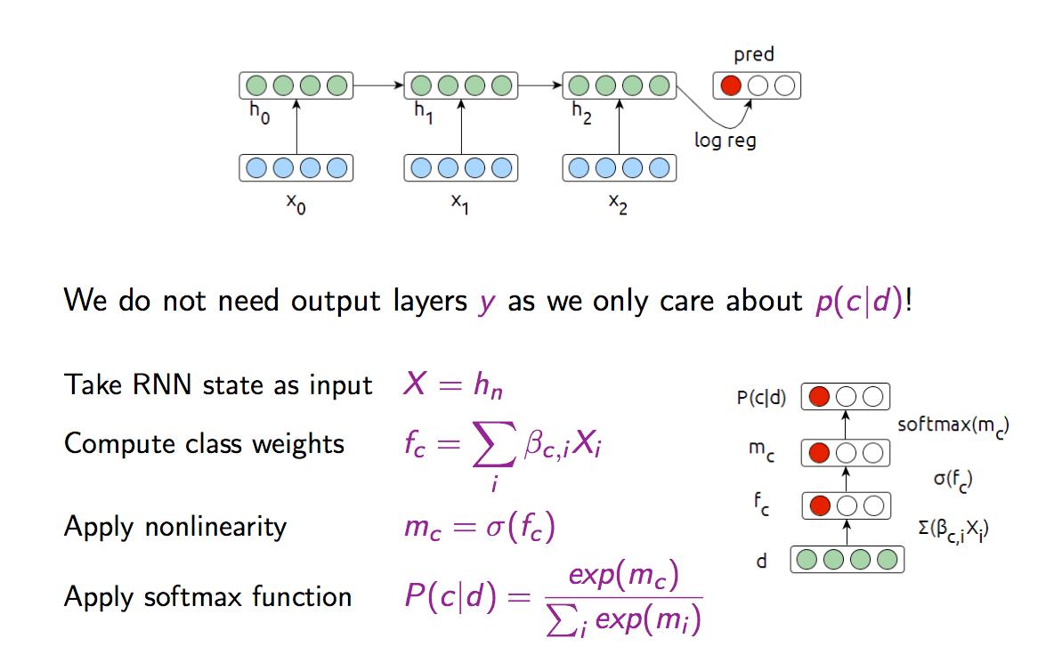
This is a simple Multilayer Perceptron (MLP). We can train the model using the cross-entropy loss: \[ L_i = -\sum_c y_c \log P(c|d_i) = -\log (\frac{\exp(m_c)}{\sum_j\exp(m_j)}) \]
- Cross-entropy is designed to deal with errors on probabilities.
- Optimizing means minimizing the cross-entropy between the estiated class probabilities (\(P(c|d)\)) and the ture distribution.
- There are many alternative losses (hinge-loss, square error, L1 loss).
Dual Objective RNN
In practice it may make sense to combine an LM objective with classifier training and to optimise the two losses jointly.
 \[
J = \alpha J_{class} + (1-\alpha)J_{lm}
\] Such a joint loss enables making use of text beyond labelled data.
\[
J = \alpha J_{class} + (1-\alpha)J_{lm}
\] Such a joint loss enables making use of text beyond labelled data.
Bi-Directional RNNs
Another way to add signal is to process the input text both in a forward and in a backward sequence.
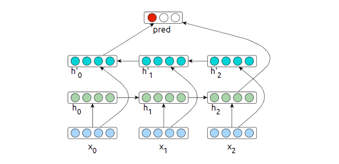
The update rules for this directly follow the regular forward-facing RNN arhitecture. In practice, bidirectional networks have shown to be more robust than unidirectional networks.
A bidirectional network can be used as a classifier simply by redefining \(d\) to be the concatenation of both final hidden states: \[ d = (\rightarrow{h_n}||h_0\leftarrow) \] RNN Classifier can be either a generative or a discriminative model
Encoder: discriminative (it does not model the probability of the text) Joint-model: generative (learns both \(P(c)\) and \(P(d)\)).
Convolutional Neural Network
Reasons to consider CNNs for Text:
- ✅ Really fast (GPU)
- ✅ BOW is often sufficient
- ✅ Actually can take some structure into account
- ❌ Not sequential in its processing of input data
- ❌ Easier to discriminate than to generate variably sized data